National Instruments NI MATRIXx Xmath Specification Sheet

Other manuals for NI MATRIXx Xmath: User Manual

Manual is about: Interactive Control Design Module

Page of 127

Download

Print this page

Bookmark us

NI MATRIXx

Xmath

Model Reduction Module

Xmath Model Reduction Module

April 2007

370755C-01

1 2 3 4 5 6 7 Next › »

Summary of NI MATRIXx Xmath

Page 1
Ni matrixx tm xmath tm model reduction module xmath model reduction module april 2007 370755c-01.
Page 2
Support worldwide technical support and product information ni.Com national instruments corporate headquarters 11500 north mopac expressway austin, texas 78759-3504 usa tel: 512 683 0100 worldwide offices australia 1800 300 800, austria 43 662 457990-0, belgium 32 (0) 2 757 0020, brazil 55 11 3262 3...
Page 3: Important Information
Important information warranty the media on which you receive national instruments software are warranted not to fail to execute programming instructions, due to defects in materials and workmanship, for a period of 90 days from date of shipment, as evidenced by receipts or other documentation. Nati...
Page 4: Conventions
Conventions the following conventions are used in this manual: [ ] square brackets enclose optional items—for example, [ response ]. Square brackets also cite bibliographic references. » the » symbol leads you through nested menu items and dialog box options to a final action. The sequence file»page...
Page 5: Contents
© national instruments corporation v xmath model reduction module contents chapter 1 introduction using this manual.........................................................................................................1-1 document organization..........................................................
Page 6
Contents xmath model reduction module vi ni.Com onepass algorithm ......................................................................................... 2-18 multipass algorithm ...................................................................................... 2-20 discrete-time systems ........
Page 7
Contents © national instruments corporation vii xmath model reduction module fracred( ) ........................................................................................................................4-15 restrictions .............................................................................
Page 8: Introduction
© national instruments corporation 1-1 xmath model reduction module 1 introduction this chapter starts with an outline of the manual and some useful notes. It also provides an overview of the model reduction module, describes the functions in this module, and introduces nomenclature and concepts use...
Page 9
Chapter 1 introduction xmath model reduction module 1-2 ni.Com • chapter 5, utilities , describes three utility functions: hankelsv( ) , stable( ) , and compare( ) . • chapter 6, tutorial , illustrates a number of the mrm functions and their underlying ideas. Bibliographic references throughout this...
Page 10: Overview
Chapter 1 introduction © national instruments corporation 1-3 xmath model reduction module related publications for a complete list of matrixx publications, refer to chapter 2, matrixx publications, online help, and customer support , of the matrixx getting started guide. The following documents are...
Page 11
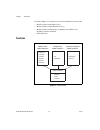
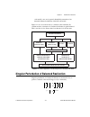
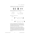
Chapter 1 introduction xmath model reduction module 1-4 ni.Com as shown in figure 1-1, functions are provided to handle four broad tasks: • model reduction with additive errors • model reduction with multiplicative errors • model reduction with frequency weighting of an additive error, including con...
Page 12
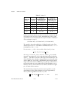
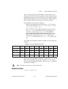
Chapter 1 introduction © national instruments corporation 1-5 xmath model reduction module certain restrictions regarding minimality and stability are required of the input data, and are summarized in table 1-1. Documentation of the individual functions sometimes indicates how the restrictions can b...
Page 13
Chapter 1 introduction xmath model reduction module 1-6 ni.Com • l 2 approximation, in which the l 2 norm of impulse response error (or, by parseval’s theorem, the l 2 norm of the transfer-function error along the imaginary axis) serves as the error measure • markov parameter or impulse response mat...
Page 14: Commonly Used Concepts
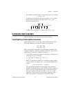
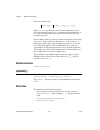
Chapter 1 introduction © national instruments corporation 1-7 xmath model reduction module • an inequality or bound is tight if it can be met in practice, for example is tight because the inequality becomes an equality for x = 1. Again, if f ( j ω ) denotes the fourier transform of some , the heisen...
Page 15
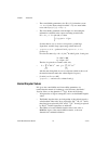
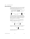
Chapter 1 introduction xmath model reduction module 1-8 ni.Com • the controllability grammian is also e [ x ( t ) x ′ ( t )] when the system has been excited from time – ∞ by zero mean white noise with . • the observability grammian can be thought of as measuring the information contained in the out...
Page 16
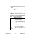
Chapter 1 introduction © national instruments corporation 1-9 xmath model reduction module • suppose the transfer-function matrix corresponds to a discrete-time system, with state variable dimension n . Then the infinite hankel matrix, has for its singular values the n nonzero hankel singular values...
Page 17
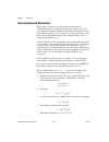
Chapter 1 introduction xmath model reduction module 1-10 ni.Com internally balanced realizations suppose that a realization of a transfer-function matrix has the controllability and observability grammian property that p = q = Σ for some diagonal Σ . Then the realization is termed internally balance...
Page 18
Chapter 1 introduction © national instruments corporation 1-11 xmath model reduction module this is almost the algorithm set out in section ii of [lhpw87]. The one difference (and it is minor) is that in [lhpw87], lower triangular cholesky factors of p and q are used, in place of u c s c 1/2 and u o...
Page 19
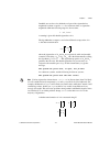
Chapter 1 introduction xmath model reduction module 1-12 ni.Com and also: re λ i ( a 22 ) and . Usually, we expect that, in the sense that the intuitive argument hinges on this, but it is not necessary. Then a singular perturbation is obtained by replacing by zero; this means that: accordingly, (1-2...
Page 20
Chapter 1 introduction © national instruments corporation 1-13 xmath model reduction module similar considerations govern the discrete-time problem, where, can be approximated by: mreduce( ) can carry out singular perturbation. For further discussion, refer to chapter 2, additive error reduction . I...
Page 21
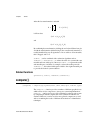
Chapter 1 introduction xmath model reduction module 1-14 ni.Com nonnegative hermitian for all ω . If Φ is scalar, then Φ ( j ω ) ≥ 0 for all ω . Normally one restricts attention to Φ (·) with lim ω→∞ Φ ( j ω ) ∞ . A key result is that, given a rational, nonnegative hermitian Φ ( j ω ) with lim ω→∞ Φ...
Page 22
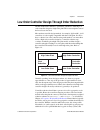
Chapter 1 introduction © national instruments corporation 1-15 xmath model reduction module low order controller design through order reduction the model reduction module is particularly suitable for achieving low order controller design for a high order plant. This section explains some of the broa...
Page 23
Chapter 1 introduction xmath model reduction module 1-16 ni.Com multiplicative reduction, as described in chapter 4, frequency-weighted error reduction , is a sound approach. Chapter 3, multiplicative error reduction , and chapter 4, frequency-weighted error reduction , develop these arguments more ...
Page 24: Additive Error Reduction
© national instruments corporation 2-1 xmath model reduction module 2 additive error reduction this chapter describes additive error reduction including discussions of truncation of, reduction by, and perturbation of balanced realizations. Introduction additive error reduction focuses on errors of t...
Page 25
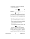
Chapter 2 additive error reduction xmath model reduction module 2-2 ni.Com truncation of balanced realizations a group of functions can be used to achieve a reduction through truncation of a balanced realization. This means that if the original system is (2-1) and the realization is internally balan...
Page 26
Chapter 2 additive error reduction © national instruments corporation 2-3 xmath model reduction module a very attractive feature of the truncation procedure is the availability of an error bound. More precisely, suppose that the controllability and observability grammians for [enn84] are (2-2) with ...
Page 27
Chapter 2 additive error reduction xmath model reduction module 2-4 ni.Com proper. So, even if all zeros are unstable, the maximum phase shift when ω moves from 0 to ∞ is (2n – 3) π /2. It follows that if g ( j ω ) remains large in magnitude at frequencies when the phase shift has moved past (2n – 3...
Page 28
Chapter 2 additive error reduction © national instruments corporation 2-5 xmath model reduction module order model is not one in general obtainable by truncation of an internally-balanced realization of the full order model. Figure 2-1 sets out several routes to a reduced-order realization. In conti...
Page 29: Hankel Norm Approximation
Chapter 2 additive error reduction xmath model reduction module 2-6 ni.Com with controllability and observability grammians given by, in which the diagonal entries of Σ are in decreasing order, that is, σ 1 ≥ σ 2 ≥ ···, and such that the last diagonal entry of Σ 1 exceeds the first diagonal entry of...
Page 30
Chapter 2 additive error reduction © national instruments corporation 2-7 xmath model reduction module function matrix. Consider the way the associated impulse response maps inputs defined over (– ∞ ,0] in l 2 into outputs, and focus on the output over [0, ∞ ). Define the input as u ( t ) for t v ( ...
Page 31: Balmoore( )
Chapter 2 additive error reduction xmath model reduction module 2-8 ni.Com further, the which is optimal for hankel norm approximation also is optimal for this second type of approximation. In xmath hankel norm approximation is achieved with ophank( ) . The most comprehensive reference is [glo84]. B...
Page 32
Chapter 2 additive error reduction © national instruments corporation 2-9 xmath model reduction module of the balanced system occurs, (assuming nsr is less than the number of states). Thus, if the state-space representation of the balanced system is with a 11 possessing dimension nsr × nsr , b 1 pos...
Page 33
Chapter 2 additive error reduction xmath model reduction module 2-10 ni.Com the actual approximation error for discrete systems also depends on frequency, and can be large at ω = 0. The error bound is almost never tight, that is, the actual error magnitude as a function of ω almost never attains the...
Page 34: Truncate( )
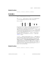
Chapter 2 additive error reduction © national instruments corporation 2-11 xmath model reduction module related functions balance() , truncate() , redschur() , mreduce() truncate( ) sysr = truncate(sys,nsr,{vd,va}) the truncate( ) function reduces a system sys by retaining the first nsr states and t...
Page 35: Redschur( )
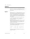
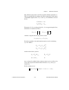
Chapter 2 additive error reduction xmath model reduction module 2-12 ni.Com redschur( ) [sysr,hsv,slbig,srbig,vd,va] = redschur(sys,{nsr,bound}) the redschur( ) function uses a schur method (from safonov and chiang) to calculate a reduced version of a continuous or discrete system without balancing....
Page 36
Chapter 2 additive error reduction © national instruments corporation 2-13 xmath model reduction module next, schur decompositions of w c w o are formed with the eigenvalues of w c w o in ascending and descending order. These eigenvalues are the square of the hankel singular values of sys , and if s...
Page 37: Ophank( )
Chapter 2 additive error reduction xmath model reduction module 2-14 ni.Com for the discrete-time case: when {bound} is specified, the error bound just enunciated is used to choose the number of states in sysr so that the bound is satisfied and nsr is as small as possible. If the desired error bound...
Page 38
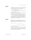
Chapter 2 additive error reduction © national instruments corporation 2-15 xmath model reduction module algorithm the algorithm does the following. The system sys and the reduced order system sysr are stable; the system sysu has all its poles in re [ s ] > 0. If the transfer function matrices are g ...
Page 39
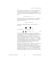
Chapter 2 additive error reduction xmath model reduction module 2-16 ni.Com by abuse of notation, when we say that g is reduced to a certain order, this corresponds to the order of g r ( s ) alone; the unstable part of g u ( s ) of the approximation is most frequently thrown away. The number of elim...
Page 40
Chapter 2 additive error reduction © national instruments corporation 2-17 xmath model reduction module thus, the penalty for not being allowed to include g u in the approximation is an increase in the error bound, by σ n i + 1 + ... + σ ns . A number of theoretical developments hinge on bounding th...
Page 41
Chapter 2 additive error reduction xmath model reduction module 2-18 ni.Com being approximated by a stable g r ( s ) with the actual error (as opposed to just the error bound) satisfying: note g r is optimal, that is, there is no other g r achieving a lower bound. Onepass algorithm the first steps o...
Page 42
Chapter 2 additive error reduction © national instruments corporation 2-19 xmath model reduction module and finally: these four matrices are the constituents of the system matrix of , where: digression: this choice is related to the ideas of [glo84] in the following way; in [glo84], the complete set...
Page 43
Chapter 2 additive error reduction xmath model reduction module 2-20 ni.Com to choose the d matrix of g r ( s ), by splitting between g r ( s ) and g u ( s ). This is done by using a separate function ophiter( ) . Suppose g u ( s ) is the unstable output of stable( ) , and let k ( s ) = g u (– s ). ...
Page 44
Chapter 2 additive error reduction © national instruments corporation 2-21 xmath model reduction module 2. Find a stable order ns – 2 approximation g ns – 2 of g ns – 1 ( s ), with 3. (step ns–nr) : find a stable order nsr approximation of g nsr + 1 , with then, because for , for , ..., this being a...
Page 45
Chapter 2 additive error reduction xmath model reduction module 2-22 ni.Com we use sysz to denote g(z) and define: bilinsys=makepoly([-1,a]/makepoly([1,a]) as the mapping from the z-domain to the s-domain. The specification is reversed because this function uses backward polynomial rotation. Hankel ...
Page 46
Chapter 2 additive error reduction © national instruments corporation 2-23 xmath model reduction module it follows by a result of [bod87] that the impulse response error for t > 0 satisfies: evidently, hankel norm approximation ensures some form of approximation of the impulse response too. Unstable...
Page 47
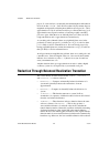
© national instruments corporation 3-1 xmath model reduction module 3 multiplicative error reduction this chapter describes multiplicative error reduction presenting two reasons to consider multiplicative rather than additive error reduction, one general and one specific. Selecting multiplicative er...
Page 48
Chapter 3 multiplicative error reduction xmath model reduction module 3-2 ni.Com multiplicative robustness result suppose c stabilizes , that has no j ω -axis poles, and that g has the same number of poles in re [ s ] ≥ 0 as . If for all ω, (3-1) then c stabilizes g . This result indicates that if a...
Page 49: Bst( )
Chapter 3 multiplicative error reduction © national instruments corporation 3-3 xmath model reduction module bandwidth at the expense of being larger outside this bandwidth, which would be preferable. Second, the previously used multiplicative error is . In the algorithms that follow, the error appe...
Page 50
Chapter 3 multiplicative error reduction xmath model reduction module 3-4 ni.Com the objective of the algorithm is to approximate a high-order stable transfer function matrix g ( s ) by a lower-order g r ( s ) with either inv(g)(g-gr) or (g-gr)inv(g) minimized, under the condition that g r is stable...
Page 51
Chapter 3 multiplicative error reduction © national instruments corporation 3-5 xmath model reduction module these cases are secured with the keywords right and left , respectively. If the wrong option is requested for a nonsquare g ( s ), an error message will result. The algorithm has the property...
Page 52
Chapter 3 multiplicative error reduction xmath model reduction module 3-6 ni.Com 2. With g ( s ) = d + c ( si – a ) –1 b and stable, with dd ´ nonsingular and g ( j ω ) g '(– j ω ) nonsingular for all ω , part of a state variable realization of a minimum phase stable w ( s ) is determined such that ...
Page 53
Chapter 3 multiplicative error reduction © national instruments corporation 3-7 xmath model reduction module strictly proper stable part of θ ( s ), as the square roots of the eigenvalues of pq . Call these quantities ν i . The schur decompositions are, where v a , v d are orthogonal and s asc , s d...
Page 54
Chapter 3 multiplicative error reduction xmath model reduction module 3-8 ni.Com state-variable representation of g . In this case, the user is effectively asking for g r = g . When the phase matrix has repeated hankel singular values, they must all be included or all excluded from the model, that i...
Page 55
Chapter 3 multiplicative error reduction © national instruments corporation 3-9 xmath model reduction module hankel singular values of phase matrix of g r the ν i , i = 1,2,..., ns have been termed above the hankel singular values of the phase matrix associated with g . The corresponding quantities ...
Page 56
Chapter 3 multiplicative error reduction xmath model reduction module 3-10 ni.Com which also can be relevant in finding a reduced order model of a plant. The procedure requires g again to be nonsingular at ω = ∞ , and to have no j ω -axis poles. It is as follows: 1. Form h = g –1 . If g is described...
Page 57
Chapter 3 multiplicative error reduction © national instruments corporation 3-11 xmath model reduction module the values of g ( s ), as shown in figure 3-2, along the j ω -axis are the same as the values of around a circle with diameter defined by [ a – j 0, b –1 + j 0] on the positive real axis. Fi...
Page 58
Chapter 3 multiplicative error reduction xmath model reduction module 3-12 ni.Com any zero (or rank reduction) on the j ω -axis of g ( s ) becomes a zero (or rank reduction) in re [ s ] > 0 of , and if g ( s ) has a zero (or rank reduction) at infinity, this is shifted to a zero (or rank reduction) ...
Page 59
Chapter 3 multiplicative error reduction © national instruments corporation 3-13 xmath model reduction module again with a bilinear transformation to secure multiplicative approximations over a limited frequency band. Suppose that create a system that corresponds to with: gtildesys=subs(gsys,(makep(...
Page 60: Mulhank( )
Chapter 3 multiplicative error reduction xmath model reduction module 3-14 ni.Com there is one potential source of failure of the algorithm. Because g ( s ) is stable, certainly will be, as its poles will be in the left half plane circle on diameter . If acquires a pole outside this circle (but stil...
Page 62
Chapter 3 multiplicative error reduction xmath model reduction module 3-16 ni.Com eigenvalues of a – b/d * c with the aid of schur( ) . If any real part of the eigenvalues is less than eps , a warning is displayed. Next, a stabilizing solution q is found for the following riccati equation: the funct...
Page 63
Chapter 3 multiplicative error reduction © national instruments corporation 3-17 xmath model reduction module singular values of f ( s ) larger than 1– ε (refer to steps 1 through 3 of the restrictions section). The maximum order permitted is the number of nonzero eigenvalues of w c w o larger than ...
Page 64
Chapter 3 multiplicative error reduction xmath model reduction module 3-18 ni.Com note the expression is the strictly proper part of . The matrix is all pass; this property is not always secured in the multivariable case when ophank( ) is used to find a hankel norm approximation of f ( s ). 5. The a...
Page 65
Chapter 3 multiplicative error reduction © national instruments corporation 3-19 xmath model reduction module • and stand in the same relation as w ( s ) and g ( s ), that is: – – with , there holds or – with there holds or – – is the stable strictly proper part of . • the hankel singular values of ...
Page 66
Chapter 3 multiplicative error reduction xmath model reduction module 3-20 ni.Com error bounds the error bound formula (equation 3-3) is a simple consequence of iterating (equation 3-5). To illustrate, suppose there are three reductions → → → , each by degree one. Then, also, similarly, then: the er...
Page 67
Chapter 3 multiplicative error reduction © national instruments corporation 3-21 xmath model reduction module for mulhank( ) , this translates for a scalar system into and the bounds are double for bst( ) . The error as a function of frequency is always zero at ω = ∞ for bst( ) (or at ω = 0 if a tra...
Page 68
Chapter 3 multiplicative error reduction xmath model reduction module 3-22 ni.Com the values of g ( s ) along the j ω -axis are the same as the values of around a circle with diameter defined by [ a – j 0, b –1 + j 0] on the positive real axis (refer to figure 3-2). Also, the values of along the j ω...
Page 69
Chapter 3 multiplicative error reduction © national instruments corporation 3-23 xmath model reduction module the error will be overbounded by the error , and g r will contain the same zeros in re [ s ] ≥ 0 as g . If there is no zero (or rank reduction) of g ( s ) at the origin, one can take a = 0 a...
Page 70
Chapter 3 multiplicative error reduction xmath model reduction module 3-24 ni.Com multiplicative approximation of (along the j ω -axis) corresponds to multiplicative approximation of g ( s ) around a circle in the right half plane, touching the j ω -axis at the origin. For those points on the j ω -a...
Page 71: Frequency-Weighted Error
© national instruments corporation 4-1 xmath model reduction module 4 frequency-weighted error reduction this chapter describes frequency-weighted error reduction problems. This includes a discussion of controller reduction and fractional representations. Introduction frequency-weighted error reduct...
Page 72
Chapter 4 frequency-weighted error reduction xmath model reduction module 4-2 ni.Com (so that ) is logical. However, a major use of weighting is in controller reduction, which is now described. Controller reduction frequency weighted error reduction becomes particularly important in reducing control...
Page 73
Chapter 4 frequency-weighted error reduction © national instruments corporation 4-3 xmath model reduction module is minimized (and of course is less than 1). Notice that these two error measures are like those of equation 4-1 and equation 4-2. The fact that the plant ought to show up in a good formu...
Page 74
Chapter 4 frequency-weighted error reduction xmath model reduction module 4-4 ni.Com most of these ideas are discussed in [enn84], [anl89], and [anm89]. The function wtbalance( ) implements weighted reduction, with five choices of error measure, namely e is , e os , e m , e ms , and e 1 with arbitra...
Page 75
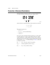
Chapter 4 frequency-weighted error reduction © national instruments corporation 4-5 xmath model reduction module fractional representations the treatment of j ω -axis or right half plane poles in the above schemes is crude: they are simply copied into the reduced order controller. A different approa...
Page 76
Chapter 4 frequency-weighted error reduction xmath model reduction module 4-6 ni.Com • form the reduced controller by interconnecting using negative feedback the second output of g r to the input, that is, set nothing has been said as to how should be chosen—and the end result of the reduction, c r ...
Page 77
Chapter 4 frequency-weighted error reduction © national instruments corporation 4-7 xmath model reduction module matrix algebra shows that c ( s ) can be described through a left or right matrix fraction description with d l , and related values, all stable transfer function matrices. In particular:...
Page 78
Chapter 4 frequency-weighted error reduction xmath model reduction module 4-8 ni.Com the left mfd corresponds to the setup of figure 4-3. Figure 4-3. C(s) implemented to display left mfd representation the setup of figure 4-2 suggests approximation of: whereas that of figure 4-3 suggests approximati...
Page 79
Chapter 4 frequency-weighted error reduction © national instruments corporation 4-9 xmath model reduction module figure 4-4. Redrawn; individual signal paths as vector paths it is possible to verify that and accordingly the output weight can be used in an error measure . It turns out that the calcul...
Page 80: Wtbalance( )
Chapter 4 frequency-weighted error reduction xmath model reduction module 4-10 ni.Com (here, the w i and v i are submatrices of w,v.) evidently, some manipulation shows that trying to preserve these identities after approximation of d l , n l or n r , d r suggests use of the error measures and . For...
Page 81
Chapter 4 frequency-weighted error reduction © national instruments corporation 4-11 xmath model reduction module • reduce the order of a transfer function matrix c ( s ) through frequency-weighted balanced truncation, a stable frequency weight v ( s ) being prescribed. The syntax is more accented t...
Page 82
Chapter 4 frequency-weighted error reduction xmath model reduction module 4-12 ni.Com this rather crude approach to the handling of the unstable part of a controller is avoided in fracred( ) , which provides an alternative to wtbalance( ) for controller reduction, at least for an important family of...
Page 83
Chapter 4 frequency-weighted error reduction © national instruments corporation 4-13 xmath model reduction module 3. Compute weighted hankel singular values σ i (described in more detail later). If the order of c r ( s ) is not specified a priori , it must be input at this time. Certain values may b...
Page 84
Chapter 4 frequency-weighted error reduction xmath model reduction module 4-14 ni.Com and the observability grammian q , defined in the obvious way, is written as it is trivial to verify that so that q cc is the observability gramian of c s ( s ) alone, as well as a submatrix of q . The weighted han...
Page 85: Fracred( )
Chapter 4 frequency-weighted error reduction © national instruments corporation 4-15 xmath model reduction module from these quantities the transformation matrices used for calculating c sr ( s ), the stable part of c r ( s ), are defined and then just as in unweighted balanced truncation, the reduc...
Page 86
Chapter 4 frequency-weighted error reduction xmath model reduction module 4-16 ni.Com 3. Only continuous systems are accepted; for discrete systems use makecontinuous( ) before calling bst( ) , then discretize the result. Sys=fracred(makecontinuous(sysd)); sysd=discretize(sys); defining and reducing...
Page 87
Chapter 4 frequency-weighted error reduction © national instruments corporation 4-17 xmath model reduction module to, for example, through, for example, balanced truncation, and then defining: for the second rationale, consider figure 4-5. Figure 4-5. Internal structure of controller recognize that ...
Page 88
Chapter 4 frequency-weighted error reduction xmath model reduction module 4-18 ni.Com controller reduction proceeds by implementing the same connection rule but on reduced versions of the two transfer function matrices. When k e has been defined through kalman filtering considerations, the spectrum ...
Page 89
Chapter 4 frequency-weighted error reduction © national instruments corporation 4-19 xmath model reduction module 6. Check the stability of the closed-loop system with c r ( s ). When the type="left perf" is specified, one works with (4-11) which is formed from the numerator and denominator of the m...
Page 90
Chapter 4 frequency-weighted error reduction xmath model reduction module 4-20 ni.Com additional background a discussion of the stability robustness measure can be found in [anm89] and [lal90]. The idea can be understood with reference to the transfer functions e ( s ) and e r ( s ) used in discussi...
Page 91
Chapter 4 frequency-weighted error reduction © national instruments corporation 4-21 xmath model reduction module the four schemes all produce different hsvs; it follows that it may be prudent to try all four schemes for a particular controller reduction. Recall again that their relative sizes are o...
Page 92: Utilities
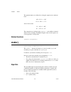
© national instruments corporation 5-1 xmath model reduction module 5 utilities this chapter describes three utility functions: hankelsv( ) , stable( ) , and compare( ) . The background to hankelsv( ) , which calculates hankel singular values, was presented in chapter 1, introduction . Hankel singul...
Page 93: Stable( )
Chapter 5 utilities xmath model reduction module 5-2 ni.Com the gramian matrices are defined by solving the equations (in continuous time) and, in discrete time the computations are effected with lyapunov( ) and stability is checked, which is time-consuming. The hankel singular values are the square...
Page 94
Chapter 5 utilities © national instruments corporation 5-3 xmath model reduction module doubtful ones are those for which the real part of the eigenvalue has magnitude less than or equal to tol for continuous-time, or eigenvalue magnitude within the following range for discrete time: a warning is gi...
Page 95: Compare( )
Chapter 5 utilities xmath model reduction module 5-4 ni.Com after this last transformation, and with it follows that and by combining the transformation yielding the real ordered schur form for a with the transformation defined using x, the overall transformation t is readily identified. In case all...
Page 96: Tutorial
© national instruments corporation 6-1 xmath model reduction module 6 tutorial this chapter illustrates a number of the mrm functions and their underlying ideas. A plant and full-order controller are defined, and then the effects of various reduction algorithms are examined. The data for this exampl...
Page 97
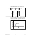
Chapter 6 tutorial xmath model reduction module 6-2 ni.Com a minimal realization in modal coordinates is c ( si – a ) –1 b where: the specifications seek high loop gain at low frequencies (for performance) and low loop gain at high frequencies (to guarantee stability in the presence of unstructured ...
Page 98
Chapter 6 tutorial © national instruments corporation 6-3 xmath model reduction module with a state weighting matrix, q = 1e-3*diag([2,2,80,80,8,8,3,3]); r = 1; (and unity control weighting), a state-feedback control-gain is determined through a linear-quadratic performance index minimization as: [k...
Page 99
Chapter 6 tutorial xmath model reduction module 6-4 ni.Com recovery at low frequencies; there is consequently a faster roll-off of the loop gain at high frequencies than for , and this is desired. Figure 6-2 displays the (magnitudes of the) plant transfer function, the compensator transfer function ...
Page 100: Controller Reduction
Chapter 6 tutorial © national instruments corporation 6-5 xmath model reduction module controller reduction this section contrasts the effect of unweighted and weighted controller reduction. Unweighted reduction is at first examined, through redschur( ) (using balance( ) or balmoore( ) will give sim...
Page 101
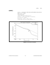
Chapter 6 tutorial xmath model reduction module 6-6 ni.Com figures 6-3, 6-4, and 6-5 display the outcome of the reduction. The loop gain is shown in figure 6-3. The error near the unity gain crossover frequency may not look large, but it is considerably larger than that obtained through frequency we...
Page 102
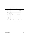
Chapter 6 tutorial © national instruments corporation 6-7 xmath model reduction module generate figure 6-4: compare(syscl,sysclr,w,{radians,type=5}) f4=plot({keep,legend=["original","reduced"]}) figure 6-4. Closed-loop gain with redschur.
Page 103
Chapter 6 tutorial xmath model reduction module 6-8 ni.Com generate figure 6-5: tvec=0:(140/99):140; compare(syscl,sysclr,tvec,{type=7}) f5=plot({keep,legend=["original","reduced"]}) figure 6-5. Step response with redschur.
Page 104
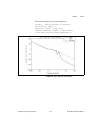
Chapter 6 tutorial © national instruments corporation 6-9 xmath model reduction module ophank( ) ophank( ) is next used to reduce the controller with the results shown in figures 6-6, 6-7, and 6-8. Generate figure 6-6: [syscr,sysu,hsv]=ophank(sysc,2); svalsrol = svplot(sys*syscr,w,{radians}); plot(s...
Page 105
Chapter 6 tutorial xmath model reduction module 6-10 ni.Com generate figure 6-7: syscl = feedback(sysol); sysolr=sys*syscr; sysclr=feedback(sysolr); compare(syscl,sysclr,w,{radians,type=5}) f7=plot({keep,legend=["original","reduced"]}) figure 6-7. Closed-loop gain with ophank.
Page 106
Chapter 6 tutorial © national instruments corporation 6-11 xmath model reduction module generate figure 6-8: tvec=0:(140/99):140; compare(syscl,sysclr,tvec,{type=7}) f8=plot({keep,legend=["original","reduced"]}) figure 6-8. Step response with ophank the open-loop gain, closed-loop gain and step resp...
Page 107
Chapter 6 tutorial xmath model reduction module 6-12 ni.Com wtbalance the next command examined is wtbalance with the option "match" . [syscr,ysclr,hsv] = wtbalance(sys,sysc,"match",2) recall that this command should promote matching of closed-loop transfer functions. The weighted hankel singular va...
Page 108
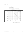
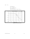
Chapter 6 tutorial © national instruments corporation 6-13 xmath model reduction module the following function calls produce figure 6-9: svalsrol = svplot(sys*syscr,w,{radians}) plot(svalsol, {keep}) f9=plot(wc, constr, {keep,!Grid, legend=["reduced","original","constrained"], title="open-loop gain ...
Page 109
Chapter 6 tutorial xmath model reduction module 6-14 ni.Com generate figure 6-10: syscl = feedback(sysol); sysolr=sys*syscr; sysclr=feedback(sysolr); compare(syscl,sysclr,w,{radians,type=5}) f10=plot({keep,legend=["original","reduced"]}) figure 6-10. Closed-loop gain with wtbalance.
Page 110
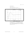
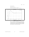
Chapter 6 tutorial © national instruments corporation 6-15 xmath model reduction module generate figure 6-11: tvec=0:(140/99):140; compare(syscl,sysclr,tvec,{type=7}) f11=plot({keep,legend=["original","reduced"]}) figure 6-11. Step response with wtbalance figures 6-9, 6-10, and 6-11 are obtained for...
Page 111
Chapter 6 tutorial xmath model reduction module 6-16 ni.Com generate figure 6-12: vtf=poly([-0.1,-10])/poly([-1,-1.4]) [,sysv]=check(vtf,{ss,convert}); svalsv = svplot(sysv,w,{radians}); figure 6-12. Frequency response of the weight v( j ω ).
Page 112
Chapter 6 tutorial © national instruments corporation 6-17 xmath model reduction module generate figure 6-13: [syscr,sysclr,hsv] = wtbalance(sys,sysc, "input spec",2,sysv) svalsrol = svplot(sys*syscr,w,{radians}) plot(svalsol, {keep}) f13=plot(wc,constr,{keep, !Grid, legend=["reduced","original","co...
Page 113
Chapter 6 tutorial xmath model reduction module 6-18 ni.Com generate figure 6-14: syscl = feedback(sysol); sysolr=sys*syscr; sysclr=feedback(sysolr); compare(syscl,sysclr,w,{radians,type=5}) f14=plot({keep,legend=["original","reduced"]}) figure 6-14. System singular values of wtbalance with "input s...
Page 114
Chapter 6 tutorial © national instruments corporation 6-19 xmath model reduction module generate figure 6-15: tvec=0:(140/99):140; compare(syscl,sysclr,tvec,{type=7}) f15=plot({keep,legend=["original","reduced"]}) figure 6-15. Step response of wtbalance with "input spec".
Page 115
Chapter 6 tutorial xmath model reduction module 6-20 ni.Com fracred fracred , the next command examined, has four options— "right stab" , "left stab" , "right perf" , and "left perf" . The options "left stab" , "right perf" , and "left perf" all produce instability. Given the relative magnitudes of ...
Page 116
Chapter 6 tutorial © national instruments corporation 6-21 xmath model reduction module generate figure 6-17: syscl = feedback(sysol); sysolr=sys*syscr; sysclr=feedback(sysolr); compare(syscl,sysclr,w,{radians,type=5}) f17=plot({keep,legend=["original","reduced"]}) figure 6-17. Closed-loop response ...
Page 117
Chapter 6 tutorial xmath model reduction module 6-22 ni.Com generate figure 6-18: tvec=0:(140/99):140; compare(syscl,sysclr,tvec,{type=7}) f18=plot({keep,legend=["original","reduced"]}) figure 6-18. Step response with fracred the end result is comparable to that from wtbalance( ) with option "match"...
Page 118
Chapter 6 tutorial © national instruments corporation 6-23 xmath model reduction module hsvtable = [... "right stab:", string(hsvrs'); "left stab:", string(hsvls'); "right perf:", string(hsvrp'); "left perf:", string(hsvlp')]? Hsvtable (a rectangular matrix of strings) = right stab:3.308 0.728 0.112...
Page 119: Bibliography
© national instruments corporation a-1 xmath model reduction module a bibliography [anj] bdo anderson and b. James, “algorithm for multiplicative approximation of a stable linear system,” in preparation. [anl89] bdo anderson and y. Liu, “controller reduction: concepts and approaches,” ieee transacti...
Page 120
Appendix a bibliography xmath model reduction module a-2 ni.Com [gra90] m. Green and bdo anderson, “generalized balanced stochastic truncation,” proceedings for 29th cdc , 1990. [gre88] m. Green, “balanced stochastic realization,” linear algebra and applications , vol. 98, 1988, pp. 211–247. [gre88a...
Page 121
Appendix a bibliography © national instruments corporation a-3 xmath model reduction module [sac88] m. G. Safonov and r. Y. Chiang, “model reduction for robust control: a schur relative-error method,” proceedings for the american controls conference , 1988, pp. 1685–1690. [saf87] m. G. Safonov, “ima...
Page 122
Appendix a bibliography xmath model reduction module a-4 ni.Com [doy82] j. C. Doyle. “analysis of feedback systems with structured uncertainties.” ieee proceedings , november 1982. [dws82] j. C. Doyle, j. E. Wall, and g. Stein. “performance and robustness analysis for structure uncertainties,” proce...
Page 123
Appendix a bibliography © national instruments corporation a-5 xmath model reduction module [slh81] m. G. Safonov, a. J. Laub, and g. L. Hartmann, “feedback properties of multivariable systems: the role and use of the return difference matrix,” ieee transactions on automatic control , vol. Ac-26, fe...
Page 124: Technical Support and
© national instruments corporation b-1 xmath model reduction module b technical support and professional services visit the following sections of the national instruments web site at ni.Com for technical support and professional services: • support —online technical support resources at ni.Com/suppo...
Page 125: Index
© national instruments corporation i-1 xmath model reduction module index symbols *, 1-6 ´, 1-6 a additive error, reduction, 2-1 algorithm balanced stochastic truncation (bst), 3-4 fractional representation reduction, 4-18 hankel multi-pass, 2-20 optimal hankel norm reduction, 2-15 stable, 5-2 weigh...
Page 126
Index xmath model reduction module i-2 ni.Com g grammians controllability, 1-7 description of, 1-7 observability, 1-7 h hankel matrix, 1-9 hankel norm approximation, 2-6 hankel singular values, 1-8, 3-9, 5-1 hankelsv, 1-5, 5-1 algorithm, multipass, 2-20 help, technical support, b-1 i instrument driv...
Page 127
Index © national instruments corporation i-3 xmath model reduction module spectral factorization, 1-13 stability requirements, 1-5 stable, 1-5, 5-2 sup, 1-6 support, technical, b-1 t technical support, b-1 tight equality bounds, 1-7 training and certification (ni resources), b-1 transfer function, a...